cs_distribution() can be used to determine the clinical
significance of intervention studies employing the distribution-based
approach. For this, the reliable change index is estimated from the
provided data and a known reliability estimate which indicates, if an
observed individual change is likely to be greater than the measurement
error inherent for the used instrument. In this case, a reliable change is
defined as clinically significant. Several methods for calculating this RCI
can be chosen.
Arguments
- data
A tidy data frame
- id
Participant ID
- time
Time variable
- outcome
Outcome variable
- group
Grouping variable (optional)
- pre
Pre measurement (only needed if the time variable contains more than two measurements)
- post
Post measurement (only needed if the time variable contains more than two measurements)
- reliability
The instrument's reliability estimate. If you selected the NK method, the here specified reliability will be the instrument's pre measurement reliability. Not needed for the HLM method.
- reliability_post
The instrument's reliability at post measurement (only needed for the NK method)
- better_is
Which direction means a better outcome for the used instrument? Available are
"lower"(lower outcome scores are desirable, the default) and"higher"(higher outcome scores are desirable)
- rci_method
Clinical significance method. Available are
"JT"(Jacobson & Truax, 1991, the default)"GLN"(Gulliksen, Lord, and Novick; Hsu, 1989, Hsu, 1995)"HLL"(Hsu, Linn & Nord; Hsu, 1989)"EN"(Edwards & Nunnally; Speer, 1992)"NK"(Nunnally & Kotsch, 1983), requires a reliability estimate at post measurement. If this is not supplied, reliability and reliability_post are assumed to be equal"HA"(Hageman & Arrindell, 1999)"HLM"(Hierarchical Linear Modeling; Raudenbush & Bryk, 2002), requires at least three measurements per patient
- significance_level
Significance level alpha, defaults to
0.05. If you choose the"HA"method, this value corresponds to the maximum risk of misclassification
Computational details
From the provided data, a region of change is calculated in which an individual change may likely be due to an inherent measurement of the used instrument. This concept is also known as the minimally detectable change (MDC).
Categories
Each individual's change may then be categorized into one of the following three categories:
Improved, the change is greater than the RCI in the beneficial direction
Unchanged, the change is within a region that may attributable to measurement error
Deteriorated, the change is greater than the RCI, but in the disadvantageous direction
Most of these methods are developed to deal with data containing two
measurements per individual, i.e., a pre intervention and post intervention
measurement. The Hierarchical Linear Modeling (rci_method = "HLM") method
can incorporate data for multiple measurements an can thus be used only
for at least three measurements per participant.
Data preparation
The data set must be tidy, which corresponds to a long data frame in general. It must contain a patient identifier which must be unique per patient. Also, a column containing the different measurements and the outcome must be supplied. Each participant-measurement combination must be unique, so for instance, the data must not contain two "After" measurements for the same patient.
Additionally, if the measurement column contains only two values, the first
value based on alphabetical, numerical or factor ordering will be used as
the pre measurement. For instance, if the column contains the
measurements identifiers "pre" and "post" as strings, then "post"
will be sorted before "pre" and thus be used as the "pre" measurement.
The function will throw a warning but generally you may want to explicitly
define the "pre" and "post" measurement with arguments pre and
post. In case of more than two measurement identifiers, you have to
define pre and post manually since the function does not know what your
pre and post intervention measurements are.
If your data is grouped, you can specify the group by referencing the grouping variable (see examples below). The analysis is then run for every group to compare group differences.
References
Jacobson, N. S., & Truax, P. (1991). Clinical significance: A statistical approach to defining meaningful change in psychotherapy research. Journal of Consulting and Clinical Psychology, 59(1), 12–19. https://doi.org/10.1037//0022-006X.59.1.12
Hsu, L. M. (1989). Reliable changes in psychotherapy: Taking into account regression toward the mean. Behavioral Assessment, 11(4), 459–467.
Hsu, L. M. (1995). Regression toward the mean associated with measurement error and the identification of improvement and deterioration in psychotherapy. Journal of Consulting and Clinical Psychology, 63(1), 141–144. https://doi.org/10.1037//0022-006x.63.1.141
Speer, D. C. (1992). Clinically significant change: Jacobson and Truax (1991) revisited. Journal of Consulting and Clinical Psychology, 60(3), 402–408. https://doi.org/10.1037/0022-006X.60.3.402
Nunnally, J. C., & Kotsch, W. E. (1983). Studies of individual subjects: Logic and methods of analysis. British Journal of Clinical Psychology, 22(2), 83–93. https://doi.org/10.1111/j.2044-8260.1983.tb00582.x
Hageman, W. J., & Arrindell, W. A. (1999). Establishing clinically significant change: increment of precision and the distinction between individual and group level analysis. Behaviour Research and Therapy, 37(12), 1169–1193. https://doi.org/10.1016/S0005-7967(99)00032-7
Raudenbush, S. W., & Bryk, A. S. (2002). Hierarchical Linear Models - Applications and Data Analysis Methods (2nd ed.). Sage Publications.
See also
Main clinical signficance functions
cs_anchor(),
cs_combined(),
cs_percentage(),
cs_statistical()
Examples
antidepressants |>
cs_distribution(patient, measurement, mom_di, reliability = 0.80)
#> ℹ Your "Before" was set as pre measurement and and your "After" as post.
#> • If that is not correct, please specify the pre measurement with the argument
#> "pre".
#>
#> ── Clinical Significance Results ──
#>
#> Distribution-based approach using the JT method.
#>
#> Category | n | Percent
#> ----------------------------
#> Improved | 274 | 49.37%
#> Unchanged | 237 | 42.70%
#> Deteriorated | 44 | 7.93%
# Turn off the warning by providing the pre measurement time
cs_results <- antidepressants |>
cs_distribution(
patient,
measurement,
mom_di,
pre = "Before",
reliability = 0.80
)
summary(cs_results)
#>
#> ── Clinical Significance Results ──
#>
#> Distribution-based analysis of clinical significance using the JT method for
#> calculating the RCI.
#>
#> There were 555 participants in the whole dataset of which 555 (100%) could be
#> included in the analysis.
#>
#> The outcome was mom_di and the reliability was set to 0.8.
#>
#>
#> ── Individual Level Results
#> Category | n | Percent
#> ----------------------------
#> Improved | 274 | 49.37%
#> Unchanged | 237 | 42.70%
#> Deteriorated | 44 | 7.93%
plot(cs_results)
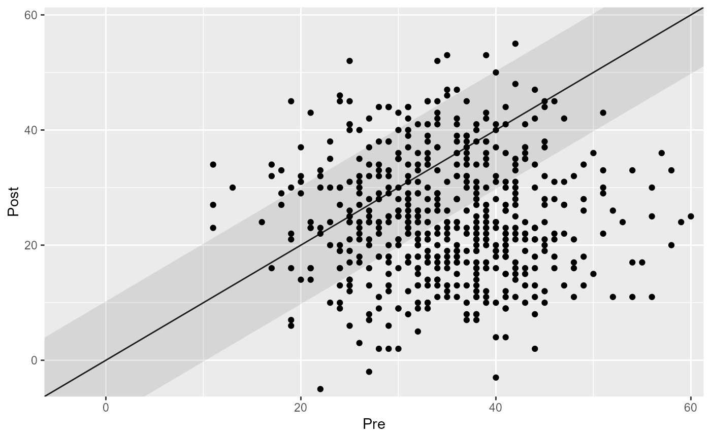 # If you use data with more than two measurements, you always have to define a
# pre and post measurement
cs_results <- claus_2020 |>
cs_distribution(
id,
time,
hamd,
pre = 1,
post = 4,
reliability = 0.80
)
cs_results
#>
#> ── Clinical Significance Results ──
#>
#> Distribution-based approach using the JT method.
#>
#> Category | n | Percent
#> ---------------------------
#> Improved | 29 | 72.50%
#> Unchanged | 10 | 25.00%
#> Deteriorated | 1 | 2.50%
summary(cs_results)
#>
#> ── Clinical Significance Results ──
#>
#> Distribution-based analysis of clinical significance using the JT method for
#> calculating the RCI.
#>
#> There were 43 participants in the whole dataset of which 40 (93%) could be
#> included in the analysis.
#>
#> The outcome was hamd and the reliability was set to 0.8.
#>
#>
#> ── Individual Level Results
#> Category | n | Percent
#> ---------------------------
#> Improved | 29 | 72.50%
#> Unchanged | 10 | 25.00%
#> Deteriorated | 1 | 2.50%
plot(cs_results)
# If you use data with more than two measurements, you always have to define a
# pre and post measurement
cs_results <- claus_2020 |>
cs_distribution(
id,
time,
hamd,
pre = 1,
post = 4,
reliability = 0.80
)
cs_results
#>
#> ── Clinical Significance Results ──
#>
#> Distribution-based approach using the JT method.
#>
#> Category | n | Percent
#> ---------------------------
#> Improved | 29 | 72.50%
#> Unchanged | 10 | 25.00%
#> Deteriorated | 1 | 2.50%
summary(cs_results)
#>
#> ── Clinical Significance Results ──
#>
#> Distribution-based analysis of clinical significance using the JT method for
#> calculating the RCI.
#>
#> There were 43 participants in the whole dataset of which 40 (93%) could be
#> included in the analysis.
#>
#> The outcome was hamd and the reliability was set to 0.8.
#>
#>
#> ── Individual Level Results
#> Category | n | Percent
#> ---------------------------
#> Improved | 29 | 72.50%
#> Unchanged | 10 | 25.00%
#> Deteriorated | 1 | 2.50%
plot(cs_results)
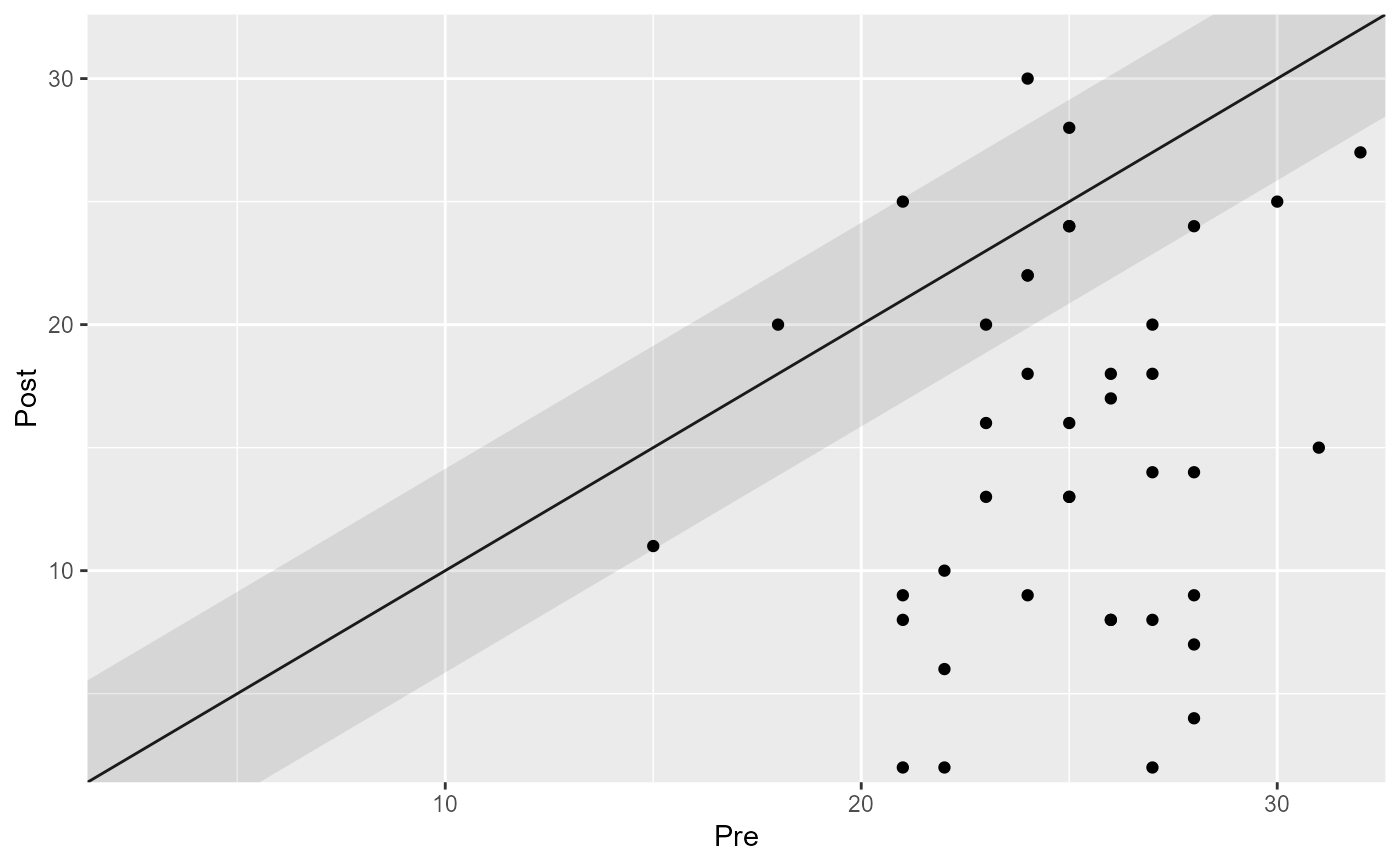 # Set the rci_method argument to change the RCI method
cs_results_ha <- claus_2020 |>
cs_distribution(
id,
time,
hamd,
pre = 1,
post = 4,
reliability = 0.80,
rci_method = "HA"
)
cs_results_ha
#>
#> ── Clinical Significance Results ──
#>
#> Distribution-based approach using the HA method.
#>
#> Category | n | Percent
#> ---------------------------
#> Improved | 32 | 80.00%
#> Unchanged | 7 | 17.50%
#> Deteriorated | 1 | 2.50%
summary(cs_results_ha)
#>
#> ── Clinical Significance Results ──
#>
#> Distribution-based analysis of clinical significance using the HA method for
#> calculating the RCI.
#>
#> There were 43 participants in the whole dataset of which 40 (93%) could be
#> included in the analysis.
#>
#> The outcome was hamd and the reliability was set to 0.8.
#>
#>
#> ── Individual Level Results
#> Category | n | Percent
#> ---------------------------
#> Improved | 32 | 80.00%
#> Unchanged | 7 | 17.50%
#> Deteriorated | 1 | 2.50%
plot(cs_results_ha)
# Set the rci_method argument to change the RCI method
cs_results_ha <- claus_2020 |>
cs_distribution(
id,
time,
hamd,
pre = 1,
post = 4,
reliability = 0.80,
rci_method = "HA"
)
cs_results_ha
#>
#> ── Clinical Significance Results ──
#>
#> Distribution-based approach using the HA method.
#>
#> Category | n | Percent
#> ---------------------------
#> Improved | 32 | 80.00%
#> Unchanged | 7 | 17.50%
#> Deteriorated | 1 | 2.50%
summary(cs_results_ha)
#>
#> ── Clinical Significance Results ──
#>
#> Distribution-based analysis of clinical significance using the HA method for
#> calculating the RCI.
#>
#> There were 43 participants in the whole dataset of which 40 (93%) could be
#> included in the analysis.
#>
#> The outcome was hamd and the reliability was set to 0.8.
#>
#>
#> ── Individual Level Results
#> Category | n | Percent
#> ---------------------------
#> Improved | 32 | 80.00%
#> Unchanged | 7 | 17.50%
#> Deteriorated | 1 | 2.50%
plot(cs_results_ha)
 # Group the analysis by providing a grouping variable
cs_results_grouped <- claus_2020 |>
cs_distribution(
id,
time,
hamd,
pre = 1,
post = 4,
group = treatment,
reliability = 0.80
)
cs_results_grouped
#>
#> ── Clinical Significance Results ──
#>
#> Distribution-based approach using the JT method.
#>
#> Group | Category | n | Percent
#> -----------------------------------
#> TAU | Improved | 9 | 22.50%
#> TAU | Unchanged | 9 | 22.50%
#> TAU | Deteriorated | 1 | 2.50%
#> PA | Improved | 20 | 50.00%
#> PA | Unchanged | 1 | 2.50%
#> PA | Deteriorated | 0 | 0.00%
summary(cs_results_grouped)
#>
#> ── Clinical Significance Results ──
#>
#> Distribution-based analysis of clinical significance using the JT method for
#> calculating the RCI.
#>
#> There were 43 participants in the whole dataset of which 40 (93%) could be
#> included in the analysis.
#>
#> The outcome was hamd and the reliability was set to 0.8.
#>
#>
#> ── Individual Level Results
#> Group | Category | n | Percent
#> -----------------------------------
#> TAU | Improved | 9 | 22.50%
#> TAU | Unchanged | 9 | 22.50%
#> TAU | Deteriorated | 1 | 2.50%
#> PA | Improved | 20 | 50.00%
#> PA | Unchanged | 1 | 2.50%
#> PA | Deteriorated | 0 | 0.00%
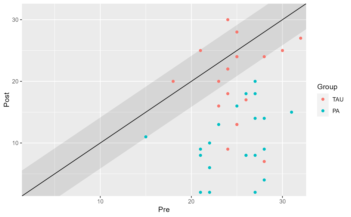
plot(cs_results_grouped)
# Group the analysis by providing a grouping variable
cs_results_grouped <- claus_2020 |>
cs_distribution(
id,
time,
hamd,
pre = 1,
post = 4,
group = treatment,
reliability = 0.80
)
cs_results_grouped
#>
#> ── Clinical Significance Results ──
#>
#> Distribution-based approach using the JT method.
#>
#> Group | Category | n | Percent
#> -----------------------------------
#> TAU | Improved | 9 | 22.50%
#> TAU | Unchanged | 9 | 22.50%
#> TAU | Deteriorated | 1 | 2.50%
#> PA | Improved | 20 | 50.00%
#> PA | Unchanged | 1 | 2.50%
#> PA | Deteriorated | 0 | 0.00%
summary(cs_results_grouped)
#>
#> ── Clinical Significance Results ──
#>
#> Distribution-based analysis of clinical significance using the JT method for
#> calculating the RCI.
#>
#> There were 43 participants in the whole dataset of which 40 (93%) could be
#> included in the analysis.
#>
#> The outcome was hamd and the reliability was set to 0.8.
#>
#>
#> ── Individual Level Results
#> Group | Category | n | Percent
#> -----------------------------------
#> TAU | Improved | 9 | 22.50%
#> TAU | Unchanged | 9 | 22.50%
#> TAU | Deteriorated | 1 | 2.50%
#> PA | Improved | 20 | 50.00%
#> PA | Unchanged | 1 | 2.50%
#> PA | Deteriorated | 0 | 0.00%
plot(cs_results_grouped)
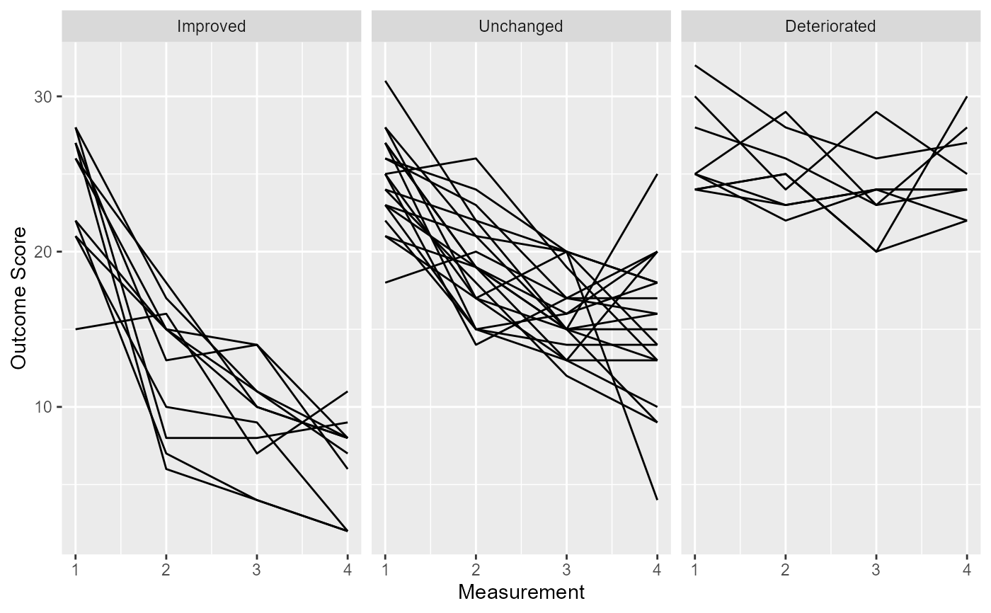
 # Use more than two measurements
cs_results_hlm <- claus_2020 |>
cs_distribution(
id,
time,
hamd,
rci_method = "HLM"
)
cs_results_hlm
#>
#> ── Clinical Significance Results ──
#>
#> Distribution-based approach using the HLM method.
#>
#> Category | n | Percent
#> ---------------------------
#> Improved | 11 | 27.50%
#> Unchanged | 20 | 50.00%
#> Deteriorated | 9 | 22.50%
summary(cs_results_hlm)
#>
#> ── Clinical Significance Results ──
#>
#> Distribution-based analysis of clinical significance using the HLM method for
#> calculating the RCI.
#>
#> There were 43 participants in the whole dataset of which 40 (93%) could be
#> included in the analysis.
#>
#> The outcome was hamd.
#>
#>
#> ── Individual Level Results
#> Category | n | Percent
#> ---------------------------
#> Improved | 11 | 27.50%
#> Unchanged | 20 | 50.00%
#> Deteriorated | 9 | 22.50%
plot(cs_results_hlm)
# Use more than two measurements
cs_results_hlm <- claus_2020 |>
cs_distribution(
id,
time,
hamd,
rci_method = "HLM"
)
cs_results_hlm
#>
#> ── Clinical Significance Results ──
#>
#> Distribution-based approach using the HLM method.
#>
#> Category | n | Percent
#> ---------------------------
#> Improved | 11 | 27.50%
#> Unchanged | 20 | 50.00%
#> Deteriorated | 9 | 22.50%
summary(cs_results_hlm)
#>
#> ── Clinical Significance Results ──
#>
#> Distribution-based analysis of clinical significance using the HLM method for
#> calculating the RCI.
#>
#> There were 43 participants in the whole dataset of which 40 (93%) could be
#> included in the analysis.
#>
#> The outcome was hamd.
#>
#>
#> ── Individual Level Results
#> Category | n | Percent
#> ---------------------------
#> Improved | 11 | 27.50%
#> Unchanged | 20 | 50.00%
#> Deteriorated | 9 | 22.50%
plot(cs_results_hlm)