Distribution-Based Approach

Introduction

In this tutorial, we will explore the percentage-change approach to clinical significance using R. The distribution-based approach is centered around the distribution of the outcome of interest. This is used to calculate the minimal detectable change (MDC), which is the change that has to be achieved to be (likely) greater than the inherent measurement error of the used instrument. We will be working with the claus_2020 dataset and the cs_percentage() function to demonstrate various aspects of these approaches.

Prerequisites

Before we begin, ensure that you have the following prerequisites in place:

R installed on your computer.
Basic understanding of R programming concepts.

Looking at the Datasets

First, let’s have a look at the datasets, which come with the package.

library(clinicalsignificance)

antidepressants
#> # A tibble: 1,110 × 4
#>    patient condition measurement mom_di
#>    <chr>   <fct>     <fct>        <dbl>
#>  1 S001    Wait List Before          50
#>  2 S001    Wait List After           36
#>  3 S002    Wait List Before          40
#>  4 S002    Wait List After           32
#>  5 S003    Wait List Before          38
#>  6 S003    Wait List After           41
#>  7 S004    Wait List Before          29
#>  8 S004    Wait List After           44
#>  9 S005    Wait List Before          37
#> 10 S005    Wait List After           45
#> # ℹ 1,100 more rows
claus_2020
#> # A tibble: 172 × 9
#>       id   age sex    treatment  time   bdi shaps   who  hamd
#>    <dbl> <dbl> <fct>  <fct>     <dbl> <dbl> <dbl> <dbl> <dbl>
#>  1     1    54 Male   TAU           1    33     9     0    25
#>  2     1    54 Male   TAU           2    28     6     3    17
#>  3     1    54 Male   TAU           3    28     9     7    13
#>  4     1    54 Male   TAU           4    27     8     3    13
#>  5     2    52 Female PA            1    26    11     2    15
#>  6     2    52 Female PA            2    26    10     0    16
#>  7     2    52 Female PA            3    25    10     0     7
#>  8     2    52 Female PA            4    19     9     3    11
#>  9     3    54 Male   PA            1    15     2     0    28
#> 10     3    54 Male   PA            2    13     5     9    17
#> # ℹ 162 more rows

The cs_distribution() function allows us to analyze the clinical significance by considering the distribution of patient measurements. We can specify various parameters to customize the analysis. Let’s explore the key aspects of this function through examples.

Basic Analysis

Let’s start with a basic clinical significance distribution analysis using the antidepressants dataset. We are interested in the Mind over Mood Depression Inventory (mom_di) measurements and want to set a reliability threshold of 0.80.

# Basic clinical significance distribution analysis
antidepressants |>
  cs_distribution(patient, measurement, mom_di, reliability = 0.80)
#> ℹ Your "Before" was set as pre measurement and and your "After" as post.
#> 
#> ── Clinical Significance Results ──
#> 
#> Distribution-based approach using the JT method.
#> • If that is not correct, please specify the pre measurement with the argument
#>   "pre".
#> Category     |   n | Percent
#> ----------------------------
#> Improved     | 274 |  49.37%
#> Unchanged    | 237 |  42.70%
#> Deteriorated |  44 |   7.93%

Handling Warnings

Sometimes, you may encounter warnings when using this function. You can turn off the warning by explicitly specifying the pre-measurement time point using the pre parameter. This can be helpful when your data lacks clear pre-post measurement labels.

# Turning off the warning by specifying pre-measurement time
cs_results <- antidepressants |>
  cs_distribution(
    patient,
    measurement,
    mom_di,
    pre = "Before",
    reliability = 0.80
  )

Summarize and plot the results

summary(cs_results)
#> 
#> ── Clinical Significance Results ──
#> 
#> Distribution-based analysis of clinical significance using the JT method for
#> calculating the RCI.
#> There were 555 participants in the whole dataset of which 555 (100%) could be
#> included in the analysis.
#> The outcome was mom_di and the reliability was set to 0.8.
#> 
#> ── Individual Level Results
#> Category     |   n | Percent
#> ----------------------------
#> Improved     | 274 |  49.37%
#> Unchanged    | 237 |  42.70%
#> Deteriorated |  44 |   7.93%
plot(cs_results)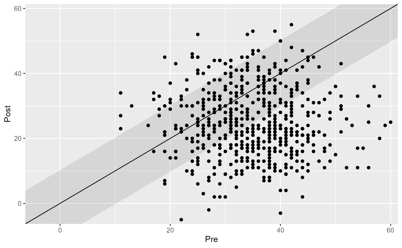

plot(cs_results, show = category)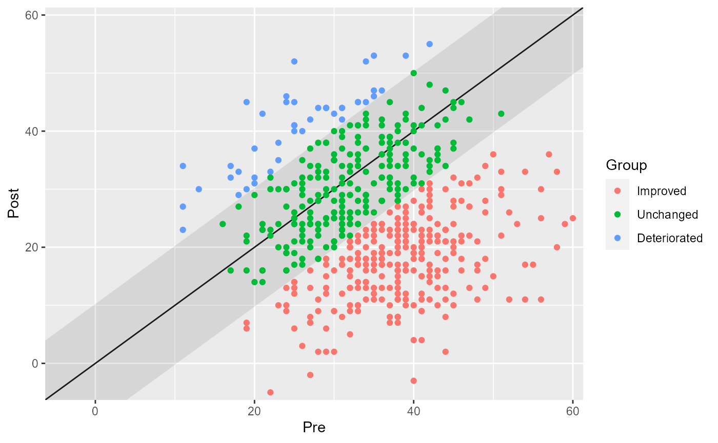

Data with More Than Two Measurements

When working with data that has more than two measurements, you must explicitly define the pre and post measurement time points using the pre and post parameters.

# Clinical significance distribution analysis with more than two measurements
cs_results <- claus_2020 |>
  cs_distribution(
    id,
    time,
    hamd,
    pre = 1,
    post = 4,
    reliability = 0.80
  )

# Display the results
cs_results
#> 
#> ── Clinical Significance Results ──
#> 
#> Distribution-based approach using the JT method.
#> Category     |  n | Percent
#> ---------------------------
#> Improved     | 29 |  72.50%
#> Unchanged    | 10 |  25.00%
#> Deteriorated |  1 |   2.50%
summary(cs_results)
#> 
#> ── Clinical Significance Results ──
#> 
#> Distribution-based analysis of clinical significance using the JT method for
#> calculating the RCI.
#> There were 43 participants in the whole dataset of which 40 (93%) could be
#> included in the analysis.
#> The outcome was hamd and the reliability was set to 0.8.
#> 
#> ── Individual Level Results
#> Category     |  n | Percent
#> ---------------------------
#> Improved     | 29 |  72.50%
#> Unchanged    | 10 |  25.00%
#> Deteriorated |  1 |   2.50%
plot(cs_results)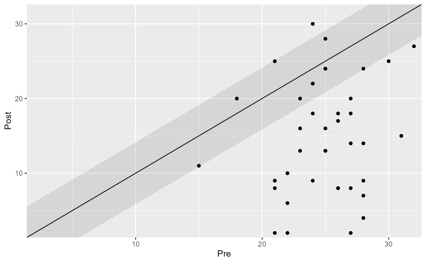

Changing the RCI Method

You can change the Reliable Change Index (RCI) method by specifying the rci_method parameter. In this example, we use the “HA” method.

# Clinical significance distribution analysis with a different RCI method
cs_results_ha <- claus_2020 |>
  cs_distribution(
    id,
    time,
    hamd,
    pre = 1,
    post = 4,
    reliability = 0.80,
    rci_method = "HA"
  )

# Display the results
summary(cs_results_ha)
#> 
#> ── Clinical Significance Results ──
#> 
#> Distribution-based analysis of clinical significance using the HA method for
#> calculating the RCI.
#> There were 43 participants in the whole dataset of which 40 (93%) could be
#> included in the analysis.
#> The outcome was hamd and the reliability was set to 0.8.
#> 
#> ── Individual Level Results
#> Category     |  n | Percent
#> ---------------------------
#> Improved     | 32 |  80.00%
#> Unchanged    |  7 |  17.50%
#> Deteriorated |  1 |   2.50%
plot(cs_results_ha)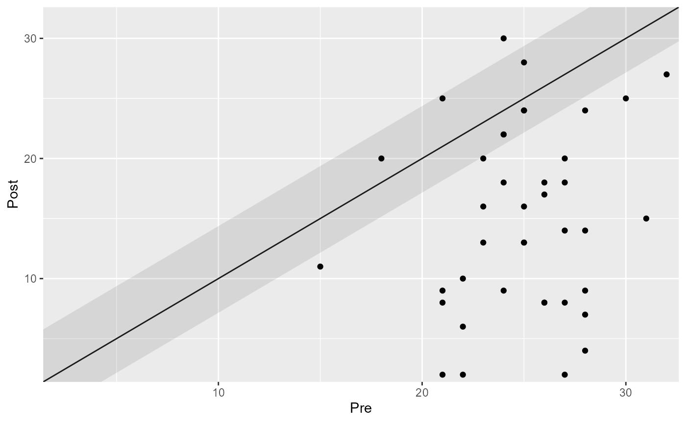

Grouped Analysis

You can also perform a grouped analysis by providing a grouping variable. This is useful when comparing different treatment groups or categories.

# Grouped analysis
cs_results_grouped <- claus_2020 |>
  cs_distribution(
    id,
    time,
    hamd,
    pre = 1,
    post = 4,
    group = treatment,
    reliability = 0.80
  )

# Display the results
summary(cs_results_grouped)
#> 
#> ── Clinical Significance Results ──
#> 
#> Distribution-based analysis of clinical significance using the JT method for
#> calculating the RCI.
#> There were 43 participants in the whole dataset of which 40 (93%) could be
#> included in the analysis.
#> The outcome was hamd and the reliability was set to 0.8.
#> 
#> ── Individual Level Results
#> Group |     Category |  n | Percent
#> -----------------------------------
#> TAU   |     Improved |  9 |  22.50%
#> TAU   |    Unchanged |  9 |  22.50%
#> TAU   | Deteriorated |  1 |   2.50%
#> PA    |     Improved | 20 |  50.00%
#> PA    |    Unchanged |  1 |   2.50%
#> PA    | Deteriorated |  0 |   0.00%
plot(cs_results_grouped)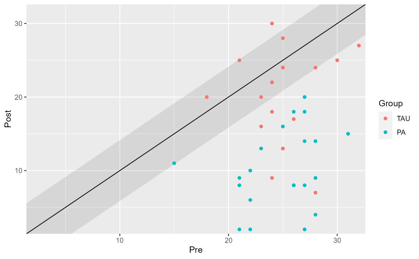

Analyzing Positive Outcomes

In some cases, higher values of an outcome may be considered better. You can specify this using the better_is argument. Let’s see an example with the WHO-5 score where higher values are considered better. Suppose the reliability for the WHO-5 is 0.85.

distribution_results_who <- claus_2020 |> 
  cs_distribution(
    id = id,
    time = time,
    outcome = who,
    pre = 1,
    post = 4,
    reliability = 0.85,
    better_is = "higher"
  )

distribution_results_who
#> 
#> ── Clinical Significance Results ──
#> 
#> Distribution-based approach using the JT method.
#> Category     |  n | Percent
#> ---------------------------
#> Improved     | 21 |  52.50%
#> Unchanged    | 18 |  45.00%
#> Deteriorated |  1 |   2.50%

# And plot the groups
plot(distribution_results_who)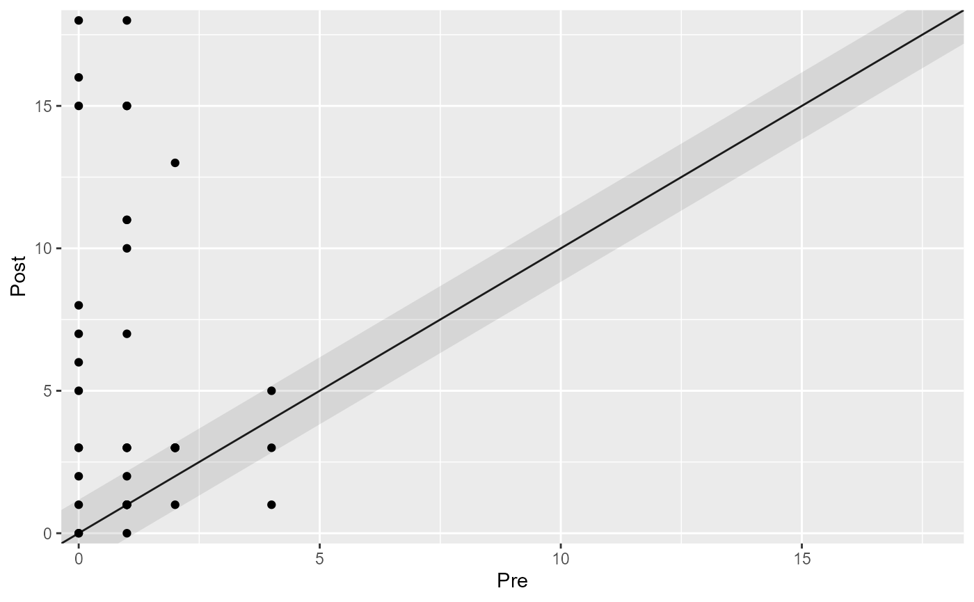

Using More Than Two Measurements with HLM Method

If you have more than two measurements and want to use the Hierarchical Linear Modeling (HLM) method, you can specify the rci_method argument accordingly.

# Clinical significance distribution analysis with HLM method
cs_results_hlm <- claus_2020 |>
  cs_distribution(
    id,
    time,
    hamd,
    rci_method = "HLM"
  )

# Display the results
summary(cs_results_hlm)
#> 
#> ── Clinical Significance Results ──
#> 
#> Distribution-based analysis of clinical significance using the HLM method for
#> calculating the RCI.
#> There were 43 participants in the whole dataset of which 40 (93%) could be
#> included in the analysis.
#> The outcome was hamd.
#> 
#> ── Individual Level Results
#> Category     |  n | Percent
#> ---------------------------
#> Improved     | 11 |  27.50%
#> Unchanged    | 20 |  50.00%
#> Deteriorated |  9 |  22.50%
plot(cs_results_hlm)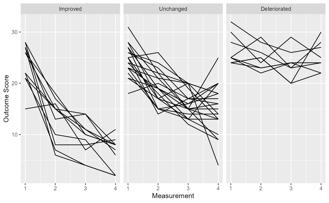

Conclusion

In this tutorial, you’ve learned how to perform clinical significance distribution analysis using the cs_distribution function in R. This analysis is valuable for understanding the practical significance of changes in patient measurements. By customizing parameters and considering group-level analysis, you can gain valuable insights for healthcare and clinical research applications.