Combined Approach • clinicalsignificance

Introduction

In this tutorial, we will explore the combined approach to clinical significance using R. The combined approaches use the anchor- or distribution-based approach in addition to the statistical approach. This is obviously stricter than the two methods on their own, but offers a more detailed interpretation. We will be working with the antidepressants and the claus_2020 datasets, and the cs_combined() function to demonstrate various aspects of this approach.

Prerequisites

Before we begin, ensure that you have the following prerequisites in place:

R installed on your computer.
Basic understanding of R programming concepts.

Looking at the Datasets

First, let’s have a look at the datasets, which come with the package.

library(clinicalsignificance)

antidepressants
#> # A tibble: 1,110 × 4
#>    patient condition measurement mom_di
#>    <chr>   <fct>     <fct>        <dbl>
#>  1 S001    Wait List Before          50
#>  2 S001    Wait List After           36
#>  3 S002    Wait List Before          40
#>  4 S002    Wait List After           32
#>  5 S003    Wait List Before          38
#>  6 S003    Wait List After           41
#>  7 S004    Wait List Before          29
#>  8 S004    Wait List After           44
#>  9 S005    Wait List Before          37
#> 10 S005    Wait List After           45
#> # ℹ 1,100 more rows
claus_2020
#> # A tibble: 172 × 9
#>       id   age sex    treatment  time   bdi shaps   who  hamd
#>    <dbl> <dbl> <fct>  <fct>     <dbl> <dbl> <dbl> <dbl> <dbl>
#>  1     1    54 Male   TAU           1    33     9     0    25
#>  2     1    54 Male   TAU           2    28     6     3    17
#>  3     1    54 Male   TAU           3    28     9     7    13
#>  4     1    54 Male   TAU           4    27     8     3    13
#>  5     2    52 Female PA            1    26    11     2    15
#>  6     2    52 Female PA            2    26    10     0    16
#>  7     2    52 Female PA            3    25    10     0     7
#>  8     2    52 Female PA            4    19     9     3    11
#>  9     3    54 Male   PA            1    15     2     0    28
#> 10     3    54 Male   PA            2    13     5     9    17
#> # ℹ 162 more rows

Claus, Wager & Bonnet Approach

This approach combines the statistical and anchor-based approach. The cs_combinedl() function is a tool for assessing clinical significance in this way. It allows you to determine if changes in patient outcomes are practically significant. Let’s go through the basic usage and some advanced features of this function.

Basic Analysis

Let’s start with a basic statistical clinical significance analysis using the antidepressants dataset. We are interested in the Mind over Mood Depression Inventory (mom_di) measurements. For the statistical approach, a functional population must be defined. Suppose, we collected data from a non-clinical sample and determined a mean of 7 points and a standard deviation of also 7 points. Furthermore, an MID of 8 points will be regarded as minimally important.

combined_results <- antidepressants |> 
  cs_combined(
    id = patient,
    time = measurement,
    outcome = mom_di,
    m_functional = 7,
    sd_functional = 7,
    cutoff_type = "c",
    mid_improvement = 8
  )
#> ℹ Your "Before" was set as pre measurement and and your "After" as post.
#> • If that is not correct, please specify the pre measurement with the argument
#>   "pre".

Handling Warnings

Sometimes, as in the example above, you may encounter warnings when using this function. You can turn off the warning by explicitly specifying the pre-measurement time point using the pre parameter. This can be helpful when your data lacks clear pre-post measurement labels.

# Turning off the warning by specifying pre-measurement time
combined_results <- antidepressants |> 
  cs_combined(
    id = patient,
    time = measurement,
    outcome = mom_di,
    pre = "Before",
    m_functional = 7,
    sd_functional = 7,
    cutoff_type = "c",
    mid_improvement = 8
  )

Here’s a breakdown of the code:

patient, measurement, and mom_di represent the patient identifier, assessment time points, and HAM-D scores, respectively.
pre and post specify the time points for the pre and post-assessment.
m_functional and sd_functional define the functional population’s mean and standard deviation. This information is used to calculate the population cutoff.
"c" specifies the population cutoff of choice.
mid_improvement sets the for improvement to 8.

Printing and Summarizing the Results

# Print the results
combined_results
#> 
#> ── Clinical Significance Results ──
#> 
#> Combined approach using the anchor-based and statistical approach.
#> Category     |   n | Percent
#> ----------------------------
#> Recovered    | 166 |  29.91%
#> Improved     | 150 |  27.03%
#> Unchanged    | 175 |  31.53%
#> Deteriorated |  52 |   9.37%
#> Harmed       |  12 |   2.16%

# Get a summary
summary(combined_results)
#> 
#> ── Clinical Significance Results ──
#> 
#> Combined analysis of clinical significance using the anchor-based and
#> statistical approach method for calculating the RCI and population cutoffs.
#> There were 555 participants in the whole dataset of which 555 (100%) could be
#> included in the analysis.
#> The outcome was mom_di and the MID was set to 8.
#> The cutoff type was c with a value of 19.72 based on the following sumamry
#> statistics:
#> 
#> ── Population Characteristics
#> M Clinical | SD Clinical | M Functional | SD Functional
#> -------------------------------------------------------
#> 34.73      |        8.26 |            7 |             7
#> 
#> ── Individual Level Results
#> Category     |   n | Percent
#> ----------------------------
#> Recovered    | 166 |  29.91%
#> Improved     | 150 |  27.03%
#> Unchanged    | 175 |  31.53%
#> Deteriorated |  52 |   9.37%
#> Harmed       |  12 |   2.16%

Visualizing the Results

Visualizing the results can help you better understand the clinical significance of changes in patient outcomes.

# Plot the results
plot(combined_results)


# Show clinical significance categories
plot(combined_results, show = category)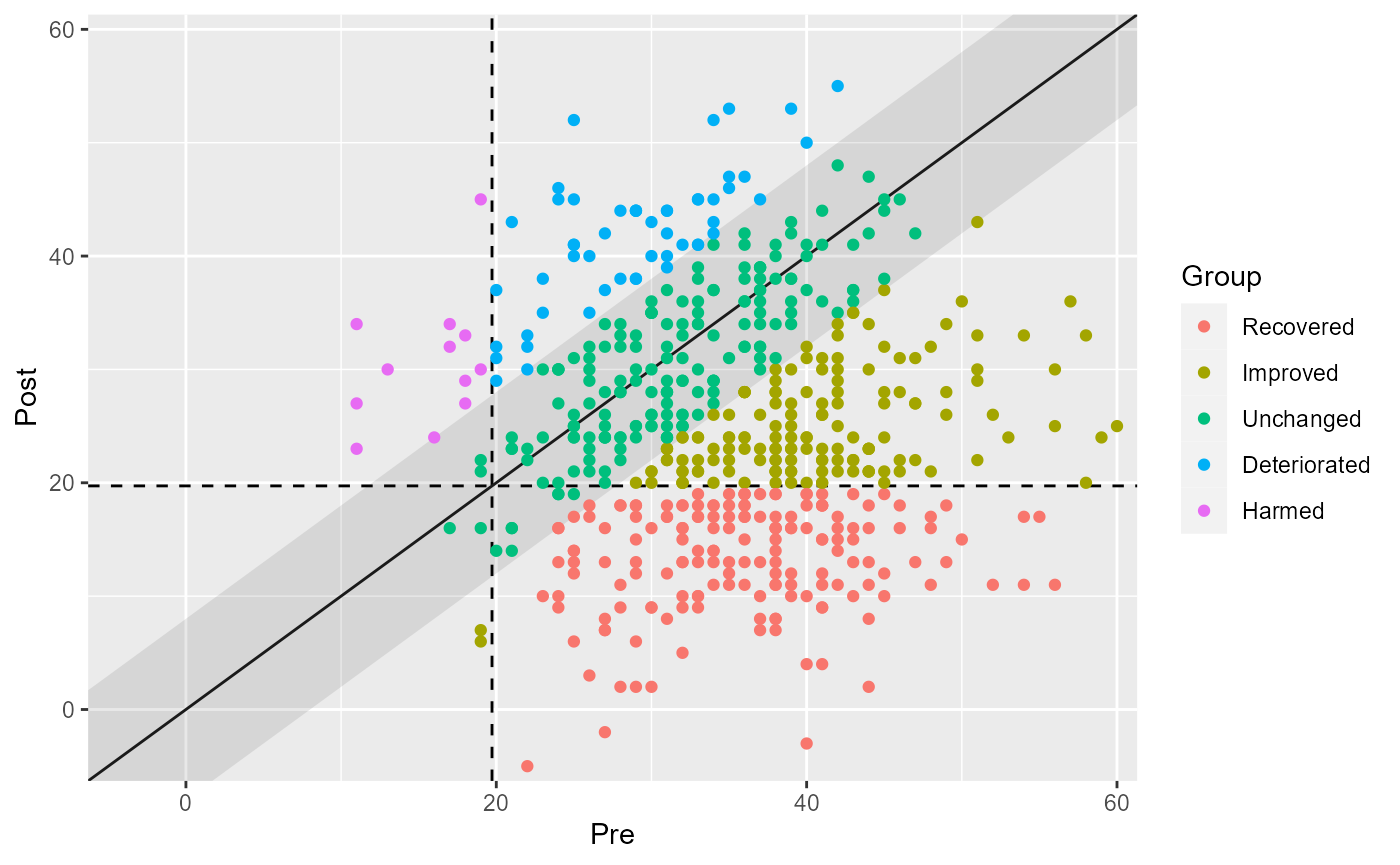

Data with More Than Two Measurements

When working with data that has more than two measurements, you must explicitly define the pre and post measurement time points using the pre and post parameters.

# Clinical significance distribution analysis with more than two measurements
cs_results <- claus_2020 |>
  cs_combined(
    id = id,
    time = time,
    outcome = bdi,
    pre = 1,
    post = 4,
    m_functional = 7,
    sd_functional = 7,
    cutoff_type = "c",
    mid_improvement = 8
  )

# Display the results
cs_results
#> 
#> ── Clinical Significance Results ──
#> 
#> Combined approach using the anchor-based and statistical approach.
#> Category     |  n | Percent
#> ---------------------------
#> Recovered    | 11 |  27.50%
#> Improved     |  9 |  22.50%
#> Unchanged    | 17 |  42.50%
#> Deteriorated |  3 |   7.50%
#> Harmed       |  0 |   0.00%
summary(cs_results)
#> 
#> ── Clinical Significance Results ──
#> 
#> Combined analysis of clinical significance using the anchor-based and
#> statistical approach method for calculating the RCI and population cutoffs.
#> There were 43 participants in the whole dataset of which 40 (93%) could be
#> included in the analysis.
#> The outcome was bdi and the MID was set to 8.
#> The cutoff type was c with a value of 20.15 based on the following sumamry
#> statistics:
#> 
#> ── Population Characteristics
#> M Clinical | SD Clinical | M Functional | SD Functional
#> -------------------------------------------------------
#> 35.48      |        8.16 |            7 |             7
#> 
#> ── Individual Level Results
#> Category     |  n | Percent
#> ---------------------------
#> Recovered    | 11 |  27.50%
#> Improved     |  9 |  22.50%
#> Unchanged    | 17 |  42.50%
#> Deteriorated |  3 |   7.50%
#> Harmed       |  0 |   0.00%
plot(cs_results)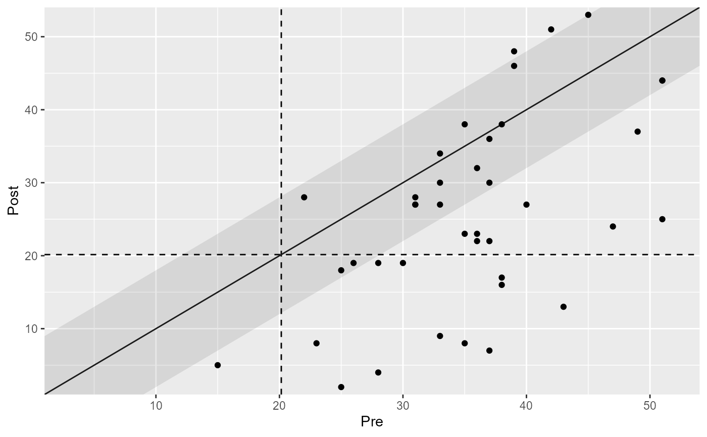

Grouped Analysis

You can also perform a grouped analysis by providing a group column from the data. This is useful when comparing treatment groups or other categories.

cs_results_grouped <- claus_2020 |>
  cs_combined(
    id = id,
    time = time,
    outcome = bdi,
    pre = 1,
    post = 4,
    m_functional = 7,
    sd_functional = 7,
    cutoff_type = "c",
    mid_improvement = 8,
    group = treatment
  )

# Display and visualize the results
cs_results_grouped
#> 
#> ── Clinical Significance Results ──
#> 
#> Combined approach using the anchor-based and statistical approach.
#> Group |     Category |  n | Percent
#> -----------------------------------
#> TAU   |    Recovered |  4 |  10.00%
#> TAU   |     Improved |  2 |   5.00%
#> TAU   |    Unchanged | 10 |  25.00%
#> TAU   | Deteriorated |  3 |   7.50%
#> TAU   |       Harmed |  0 |   0.00%
#> PA    |    Recovered |  7 |  17.50%
#> PA    |     Improved |  7 |  17.50%
#> PA    |    Unchanged |  7 |  17.50%
#> PA    | Deteriorated |  0 |   0.00%
#> PA    |       Harmed |  0 |   0.00%
plot(cs_results_grouped)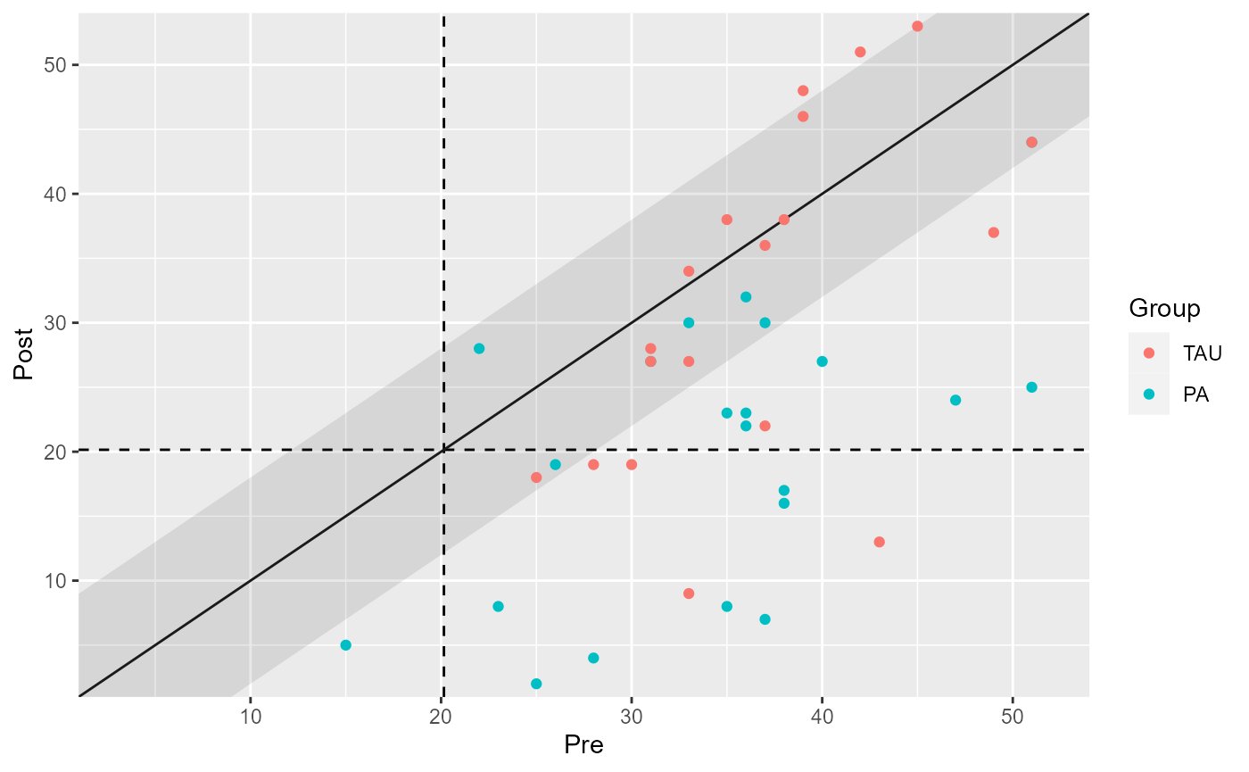

Analyzing Positive Outcomes

In some cases, higher values of an outcome may be considered better. You can specify this using the better_is argument. Let’s see an example with the WHO-5 score where higher values are considered better.

# Clinical significance analysis for outcomes where higher values are better
cs_results_who <- claus_2020 |>
  cs_combined(
    id,
    time,
    who,
    pre = 1,
    post = 4,
    m_functional = 7,
    sd_functional = 7,
    cutoff_type = "c",
    mid_improvement = 8,
    better_is = "higher"
  )

# Display the results
cs_results_who
#> 
#> ── Clinical Significance Results ──
#> 
#> Combined approach using the anchor-based and statistical approach.
#> Category     |  n | Percent
#> ---------------------------
#> Recovered    | 10 |  25.00%
#> Improved     |  1 |   2.50%
#> Unchanged    | 29 |  72.50%
#> Deteriorated |  0 |   0.00%
#> Harmed       |  0 |   0.00%

Jacobson & Truax Approach

The Jacobson & Truax approach combines the statistical with the distribution-based approach. For this, let’s suppose that the reliability of the MoM-DI is 0.80.

jt_results <- antidepressants |> 
  cs_combined(
    id = patient,
    time = measurement,
    outcome = mom_di,
    pre = "Before",
    m_functional = 7,
    sd_functional = 7,
    cutoff_type = "c",
    reliability = 0.80
  )

# Summarize and visualize the results
summary(jt_results)
#> 
#> ── Clinical Significance Results ──
#> 
#> Combined analysis of clinical significance using the JT and statistical
#> approach method for calculating the RCI and population cutoffs.
#> There were 555 participants in the whole dataset of which 555 (100%) could be
#> included in the analysis.
#> The outcome was mom_di and the reliability was set to 0.8.
#> The cutoff type was c with a value of 19.72 based on the following sumamry
#> statistics:
#> 
#> ── Population Characteristics
#> M Clinical | SD Clinical | M Functional | SD Functional
#> -------------------------------------------------------
#> 34.73      |        8.26 |            7 |             7
#> 
#> ── Individual Level Results
#> Category     |   n | Percent
#> ----------------------------
#> Recovered    | 159 |  28.65%
#> Improved     | 115 |  20.72%
#> Unchanged    | 237 |  42.70%
#> Deteriorated |  34 |   6.13%
#> Harmed       |  10 |   1.80%
plot(jt_results)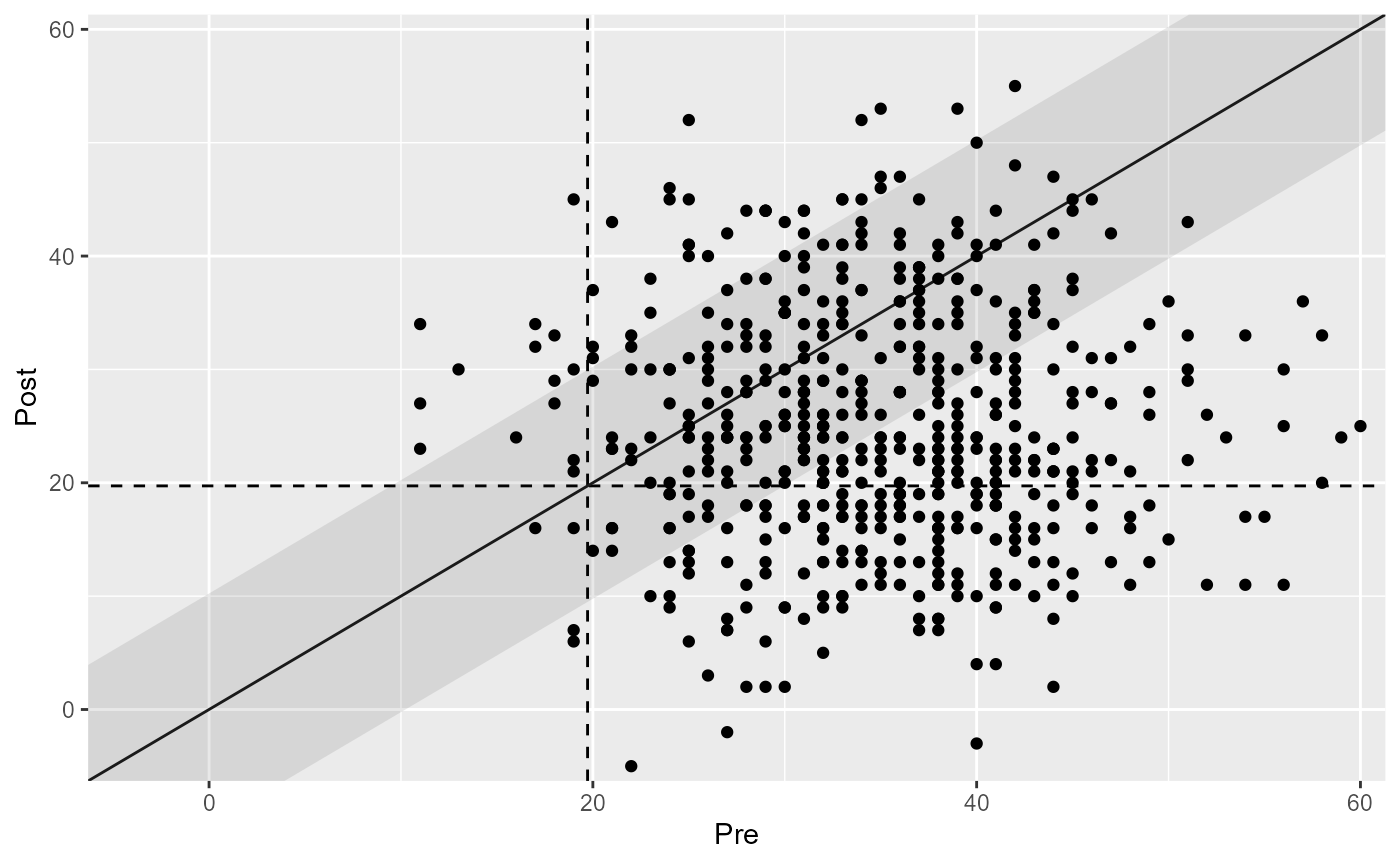

plot(jt_results, show = category)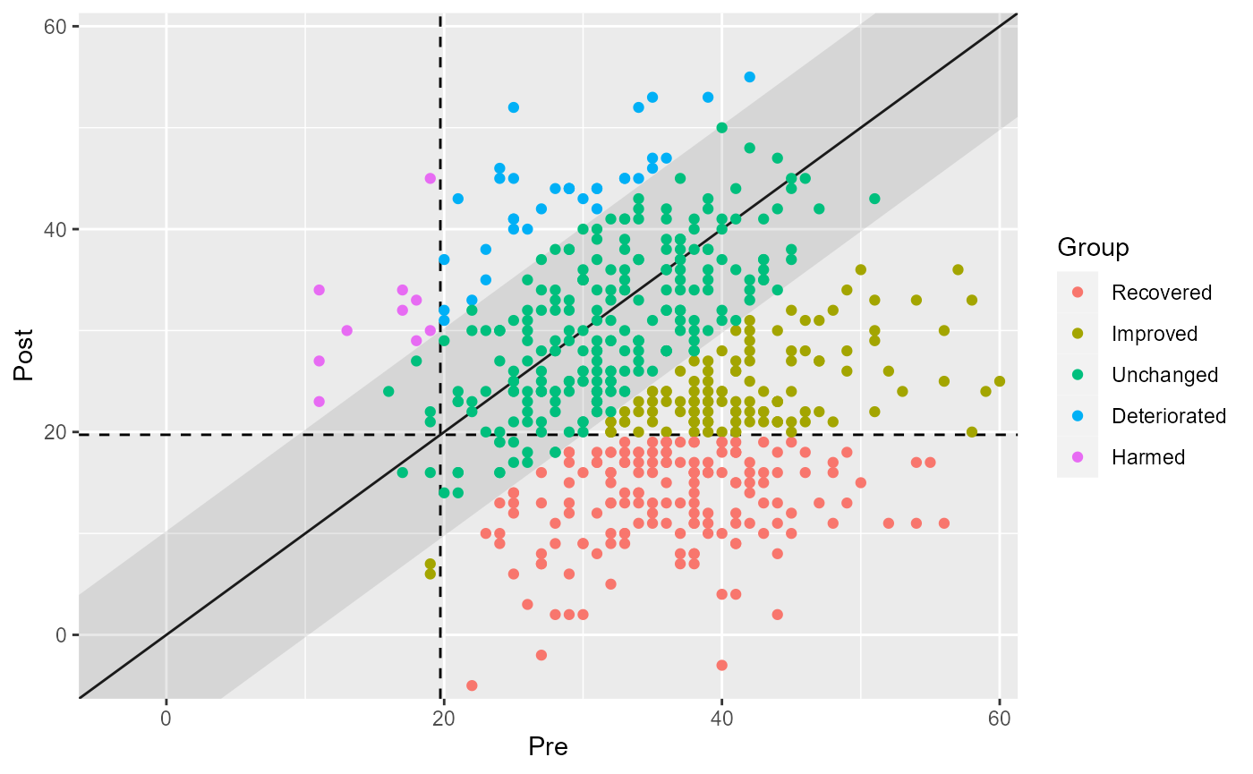

Conclusion

In this tutorial, you’ve learned how to perform clinical significance analysis using the cs_combined() function in R. This analysis may be crucial for determining the practical importance of changes in patient outcomes. By adjusting thresholds and considering grouped analyses, you can gain valuable insights for healthcare and clinical research applications.